

Part 6 of my series on Craig Freedman’s SQL Server query-processing blog (part 5, October 2006, is here). November 2006 puts the exchange operator from last month to work: how scans, nested loops joins and hash joins actually run in parallel, and then a first look at partitioned tables. Summaries in my own words; the mechanics are unchanged in modern SQL Server.
All plan screenshots in this post are my own, made in SSMS with “Include Actual Execution Plan” (Ctrl+M). Want to follow along? Run this one-time setup in a scratch database (it uses GENERATE_SERIES, so SQL Server 2022 or later) — the cleanup is at the bottom of the post. Fair warning: the two big tables are a million rows each (~500 MB together, a minute or two of loading) — parallelism needs something worth parallelizing:
-- One-time setup for the examples in this post
CREATE TABLE dbo.T1 (a INT, b INT, x CHAR(200));
INSERT dbo.T1 SELECT value, value, value FROM GENERATE_SERIES(0, 999999);

SELECT * INTO dbo.T2 FROM dbo.T1;
CREATE UNIQUE CLUSTERED INDEX T2a ON dbo.T2 (a);

CREATE PARTITION FUNCTION pf (INT) AS RANGE FOR VALUES (0, 10, 100);
CREATE PARTITION SCHEME ps AS PARTITION pf ALL TO ([PRIMARY]);
CREATE TABLE dbo.pt (a INT, b INT) ON ps (a);
INSERT dbo.pt SELECT value, value FROM GENERATE_SERIES(-50, 149);24. Parallel Scan (November 2, 2006)
The scan is one of the few operators that is genuinely parallel-aware. There is no fixed assignment of pages to threads: a parallel page supplier in the storage engine hands out batches of pages on demand, each page to exactly one thread. That design has two lovely properties — it works for any number of threads without recompiling anything, and it load-balances automatically: a slow thread simply asks for fewer pages while faster threads pick up the slack. Craig proves it with statistics XML: on an idle box two threads each scan ~50% of a million rows, but with a CPU-hogging serial query running alongside, the free thread takes over 90% of the pages by itself.
Also worth noting: a bare SELECT * FROM T over a million rows gets a serial plan. Parallelism is about spending more CPU, and a plain scan is I/O- and network-bound; add a predicate worth evaluating and the parallel plan appears. And in the per-thread output, thread 0 always shows zero rows — that’s the coordinator, which only runs the plan above the top exchange.
Add that predicate and the parallel plan appears — the little yellow double-arrow badges on the operators mark the parallel zone, with Gather Streams funneling everything back to the coordinator. Open the Table Scan’s properties and check “Actual Number of Rows” per thread to see the load balancing live:
SELECT * FROM dbo.T1 WHERE a < 1000;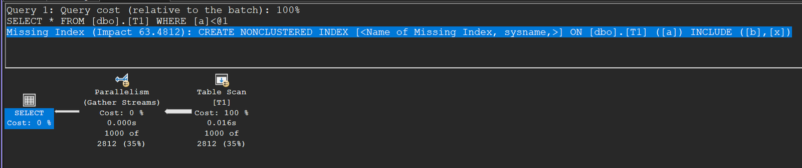
25. Parallel Nested Loops Join (November 8, 2006)
A nested loops join is parallelized on its outer side only: the outer rows are distributed across threads (usually just by the parallel scan itself — note there’s often only a single Gather Streams at the root of such plans), and each thread runs the entire inner side serially for its own rows, with its own correlated parameters. The inner side of a nested loops join is never parallelized, no matter how complex it is.
Here’s the shape on the million-row tables: one Gather Streams at the root, a parallel Table Scan of T1 on the outer side (my run adds a Repartition Streams exchange to spread the 100 qualifying rows across threads), and each thread driving its own serial Clustered Index Seeks into T2:
SELECT * FROM dbo.T1 JOIN dbo.T2 ON T1.b = T2.a WHERE T1.a < 100;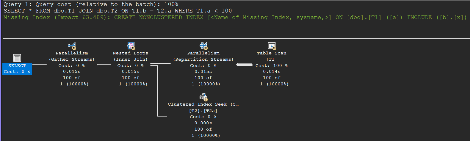
When the parallel scan can’t do the distribution — say a TOP sits on the outer side, which only works correctly in a single thread — the plan adds a Round Robin Distribute Streams exchange to spread the rows. The trade-off Craig highlights: round robin doesn’t load-balance the way the parallel scan does, and both can leave threads idle when there are few rows. His own example shows it: with a predicate matching only the first 100 rows of the table, all the qualifying pages land on one thread and the second join thread does exactly nothing — invisible unless you check the per-thread row counts.
26. Parallel Hash Join (November 16, 2006)
Hash joins parallelize with one of two strategies. The common one is hash partitioning: Repartition Streams exchanges on both inputs hash-distribute build and probe rows on the join keys, so matching rows are guaranteed to land on the same thread and the join instances run fully independently — the reason hash join scales so well. The alternative is the broadcast hash join: when the build side is small, every build row is sent to every thread, and the probe rows can then go anywhere (usually straight from the parallel scan, no second exchange needed). Broadcast eliminates skew risk, but at a price: memory grows linearly with DOP, because each thread holds a full copy of the hash table.
An honest footnote from reproducing this in 2026: on my SQL Server 2022 instance neither textbook shape materializes. The big join below runs parallel (note the badges), but without Repartition Streams on the inputs — and the selective variant below it shows no Distribute Streams either. The likely reason is batch mode on rowstore, where all threads share a single hash table and no row shuffling is needed (check “Actual Execution Mode” in the operator properties). The exchange taxonomy is still exactly what you’ll see in row-mode plans — the nested loops example above has one — but it’s a nice illustration of how execution kept evolving after 2006:
SELECT COUNT(*) FROM dbo.T1 JOIN dbo.T2 ON T1.b = T2.b;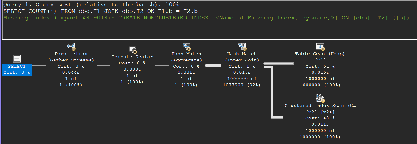
SELECT * FROM dbo.T1 JOIN dbo.T2 ON T1.b = T2.b WHERE T1.a = 0;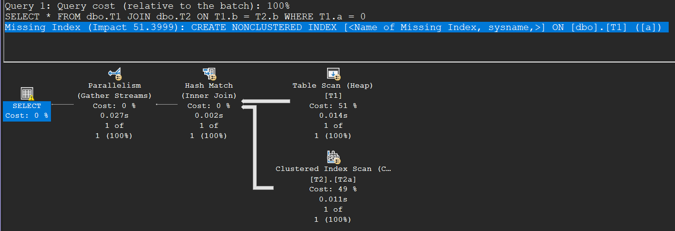
The article closes with the Bitmap operator: with a selective filter on the build side, the join builds a bitmap of the surviving join-key hashes and pushes it into the exchange above the probe scan, so probe rows that can’t possibly join are discarded before they ever travel through the exchange to the join. That’s the ancestor of the bitmap filters you see in every large parallel plan (and, conceptually, of batch-mode bloom filters) — semi-join reduction in action.
27. Introduction to Partitioned Tables (November 27, 2006)
The SQL Server 2005 way of executing partitioned-table plans looks odd at first sight and this article decodes it: a scan of a four-partition table shows up as a Constant Scan listing the partition IDs, nested-loops-joined to the actual table scan, which runs once per partition. From there, three flavors of partition elimination:
- Static elimination: a literal predicate like
a < 100removes partitions from the Constant Scan at compile time; if only one partition survives, the join scaffolding disappears entirely. - Dynamic elimination: with a parameter (
a < @i) the partition list can’t be known at compile time, so a Filter with the internalRangePartitionNewfunction trims the partition IDs at run time. - Combined:
a > 0 AND a < @istatically drops partition 1 and dynamically filters the rest.
On a modern SQL Server you won’t see the Constant Scan scaffolding anymore — the 2008+ plan shape below is a single scan with a hidden seek predicate on the partition id (look at the seek predicate and “Actual Partition Count” in the properties). But both eliminations still happen exactly as described: the literal predicate touches three partitions and returns all 150 qualifying rows; the variable version decides at run time and returns only the 50 rows of the surviving partition:
SELECT * FROM dbo.pt WHERE a < 100;

DECLARE @i INT = 0;
SELECT * FROM dbo.pt WHERE a < @i;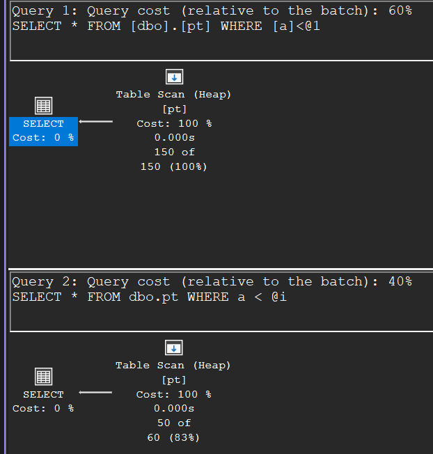
You can invoke the partition mapping yourself with $partition.pf(a). One warning from the closing notes still applies: OR-predicates involving parameters can defeat partition elimination altogether — sometimes a UNION rewrite is the workaround. (In SQL Server 2008 the plan shape changed to per-operator partitioning info, but the elimination concepts here carried straight over.)
Done experimenting? This removes everything the setup created:
-- Cleanup
DROP TABLE IF EXISTS dbo.T1, dbo.T2, dbo.pt;
DROP PARTITION SCHEME ps;
DROP PARTITION FUNCTION pf;