

Back in June 2006, Craig Freedman — at the time a developer on the SQL Server query processing team at Microsoft — started a blog about how SQL Server actually executes queries. Almost twenty years later it is still one of the best places to learn how to read execution plans, because it was written by someone who worked on the engine itself. Microsoft has preserved the blog in its archive on learn.microsoft.com, but it is easy to overlook there, and the original ordering is what makes it work as a course.
With this post I’m starting a series that walks through Craig’s articles month by month, in the order he wrote them. This first part covers the six articles from June 2006 — the foundations: what a query plan is made of, how to look at one, and the scan/seek/lookup trio that every DBA runs into daily. For each article I summarize the core ideas in my own words. Everything described here still applies to modern SQL Server versions.
All plan screenshots in this post are my own, made in SSMS with “Include Actual Execution Plan” (Ctrl+M). Want to follow along? Run this one-time setup in a scratch database (it uses GENERATE_SERIES, so SQL Server 2022 or later) — the cleanup is at the bottom of the post:
-- One-time setup for the examples in this post
CREATE TABLE dbo.t (a INT);
INSERT dbo.t SELECT value FROM GENERATE_SERIES(1, 1000);

CREATE TABLE dbo.t1 (a INT);
CREATE TABLE dbo.t2 (a INT);
INSERT dbo.t1 SELECT value FROM GENERATE_SERIES(1, 100);
INSERT dbo.t2 SELECT value FROM GENERATE_SERIES(1, 100);

CREATE TABLE dbo.Orders (OrderKey INT, OrderDate DATE);
INSERT dbo.Orders
SELECT value, DATEADD(DAY, value % 365, '20260101') FROM GENERATE_SERIES(1, 10000);

CREATE TABLE dbo.T_clu (a INT, b INT, c INT, d INT, e INT);
CREATE UNIQUE CLUSTERED INDEX T_clu_a ON dbo.T_clu (a);
CREATE INDEX T_clu_b ON dbo.T_clu (b);
INSERT dbo.T_clu SELECT value, value, value, value, value FROM GENERATE_SERIES(1, 1000);

CREATE TABLE dbo.T_heap (a INT, b INT, c INT, d INT, e INT);
CREATE INDEX T_heap_a ON dbo.T_heap (a);
INSERT dbo.T_heap SELECT value, value, value, value, value FROM GENERATE_SERIES(1, 1000);1. Why am I starting this blog? (June 7, 2006)
A short kickoff post. Craig explains that the blog grew out of user group talks he gave about how SQL Server executes queries — reading showplan output and understanding common operators like scans, seeks, joins and aggregation — and that he wants to capture those topics in writing. Short as it is, it sets the agenda for everything that follows.
2. The Building Blocks of Query Execution (June 8, 2006)
This is the article that gives you the mental model for everything else. SQL Server compiles every query into a tree of iterators (also called operators). Each iterator does exactly one job — scan a table, filter rows, join two inputs, aggregate — and there are only a few dozen of them. Because they all expose the same interface (essentially Open, GetRow and Close), they can be snapped together into arbitrary trees: the query plans you see in Management Studio.
The key insight is the direction of flow: control flows down the tree (the root iterator asks its children for rows), while data is pulled up, one row at a time. Craig illustrates this with the simplest possible query, a SELECT COUNT(*), which is just a stream aggregate sitting on top of a table scan: the aggregate keeps calling GetRow on the scan and counts what comes back. Here is that exact plan in a modern SSMS — Table Scan feeding a Stream Aggregate (the Compute Scalar just converts the bigint count to int):
SELECT COUNT(*) FROM dbo.t;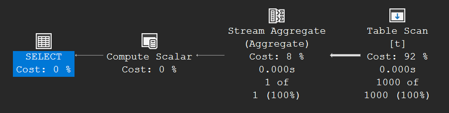
Once you see plans as iterator trees with rows being pulled upward, plan reading stops being intimidating.
3. Viewing Query Plans (June 13, 2006)
Now that you know queries become iterator trees, how do you look at them? Craig walks through the three showplan formats — graphical, text and XML — and their trade-offs: graphical is great for the big picture, text is easier to save, search and compare (especially for large plans), and XML combines the strengths of both and is what the .sqlplan files really are.
He also makes a distinction that still confuses people today: the estimated execution plan (compiled without running the query, useful for long-running statements or for DML you don’t want to execute) versus the actual execution plan, which adds real row counts you can compare against the estimates. The article includes a handy reference of the old SET options (SHOWPLAN_TEXT, SHOWPLAN_ALL, STATISTICS PROFILE, SHOWPLAN_XML, STATISTICS XML) and which of them execute the query and which don’t — worth bookmarking on its own.
Craig’s example of an operator with two children is a simple UNION ALL of two tables — two Table Scans feeding a Concatenation operator, which makes the tree structure of a plan immediately visible:
SELECT a FROM dbo.t1
UNION ALL
SELECT a FROM dbo.t2;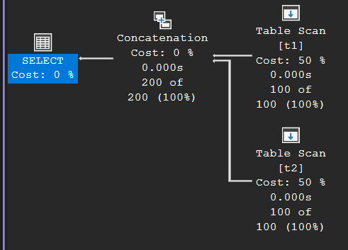
4. Properties of Iterators (June 19, 2006)
Not all iterators behave the same, and Craig highlights three properties with direct performance impact:
- Memory consumption. Most iterators need only a small fixed amount of memory, but sort, hash join and hash aggregate need memory proportional to the data they process. That is why queries with these operators need a memory grant before they can start — they may have to wait for one, and if the grant turns out too small they spill to tempdb, which can hurt badly. Anyone who has chased memory grant waits or tempdb spills in Query Store will recognize how current this 2006 list still is.
- Blocking vs. non-blocking. Non-blocking iterators (like compute scalar) produce output while they consume input; blocking (“stop-and-go”) iterators (like sort) must consume all input before producing the first output row. For OLTP workloads and
TOP Nqueries you want non-blocking plans — and Craig drops the practical hint that the right index can let the optimizer avoid a blocking sort entirely because the index already delivers the desired order. - Dynamic cursor support. A dynamic cursor plan can only use iterators that can save/restore state, scan in both directions and stay non-blocking — which is why some queries simply cannot run as a dynamic cursor.
5. Scans vs. Seeks (June 26, 2006)
The most quoted article of the month, and rightly so. Craig’s definition is beautifully compact: “A scan returns the entire table or index. A seek efficiently returns rows from one or more ranges of an index based on a predicate.”
The cost model follows directly: a scan touches every row whether it qualifies or not, so its cost is proportional to the size of the table; a seek only touches qualifying rows and pages, so its cost is proportional to the result, not the table. That also means a scan is not automatically bad — for a small table, or a predicate that most rows satisfy anyway, a scan is the right choice.
Here are both shapes for the same query on an Orders table. Without an index, a Table Scan that reads everything and filters:
SELECT OrderDate FROM dbo.Orders WHERE OrderKey = 2;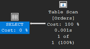
And with an index on OrderKey, an Index Seek that goes straight to the qualifying row:
CREATE INDEX OKEY_IDX ON dbo.Orders (OrderKey) INCLUDE (OrderDate);

SELECT OrderDate FROM dbo.Orders WHERE OrderKey = 2;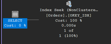
Two vocabulary items from this article that you’ll use forever: a residual predicate (the WHERE: in showplan) is evaluated against every row a scan reads, while a seek predicate (the SEEK: keyword) is used to navigate the index directly. He closes with the little matrix of operator names — Table Scan for heaps, Clustered Index Scan/Seek, and Index Scan/Seek for non-clustered indexes — that decodes what you see in every plan.
6. Bookmark Lookup (June 30, 2006)
The June finale connects seeks to indexing strategy. A non-clustered index covers only its key columns, the clustering keys, and (since SQL Server 2005) any INCLUDEd columns. If a query needs a column the index does not cover, SQL Server seeks the non-clustered index and then follows a bookmark — a pointer to the base table row — to fetch the missing columns. In modern plans that shows up as a nested loops join to a Key Lookup (clustered index seek with the LOOKUP keyword):
SELECT e FROM dbo.T_clu WITH (INDEX(T_clu_b)) WHERE b = 2;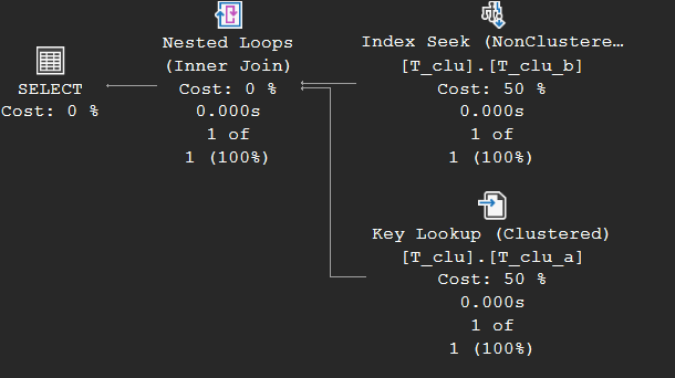
Or, when the base table is a heap, as a RID Lookup:
SELECT e FROM dbo.T_heap WITH (INDEX(T_heap_a)) WHERE a = 2;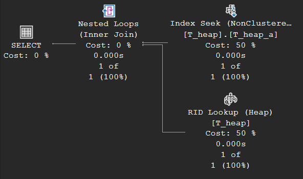
Done experimenting? This removes everything the setup created:
-- Cleanup
DROP TABLE IF EXISTS dbo.t, dbo.t1, dbo.t2, dbo.Orders, dbo.T_clu, dbo.T_heap;The performance warning is the part every DBA should internalize: each lookup is effectively a random I/O against the base table, so a seek plus thousands of lookups can easily be slower than a single scan. That is exactly the trade-off the optimizer weighs, and it is why adding an INCLUDE column to make an index covering is such a common and effective tuning move — balanced, as Craig notes, against the extra disk space and maintenance cost of widening the index.