

This is part 2 of my series on Craig Freedman’s classic SQL Server query-processing blog (part 1, June 2006, is here). In July 2006 Craig published four articles that finish the story of indexes and access paths, and then open the biggest chapter of the whole blog: joins. As before, I summarize the core ideas of each article in my own words — and as before, every word of it still applies to modern SQL Server versions.
All plan screenshots in this post are my own, made in SSMS with “Include Actual Execution Plan” (Ctrl+M). Want to follow along? Run this one-time setup in a scratch database (it uses GENERATE_SERIES, so SQL Server 2022 or later) — the cleanup is at the bottom of the post:
-- One-time setup for the examples in this post
CREATE TABLE dbo.person (id INT, last_name VARCHAR(30), first_name VARCHAR(30));
CREATE UNIQUE CLUSTERED INDEX person_id   ON dbo.person (id);
CREATE NONCLUSTERED INDEX    person_name ON dbo.person (last_name, first_name);
INSERT dbo.person
SELECT value,
       CHAR(65 + value % 26) + 'name' + CAST(value % 100 AS VARCHAR(3)),
       CHAR(65 + value % 26) + CAST(value AS VARCHAR(6))
FROM GENERATE_SERIES(1, 5000);

CREATE TABLE dbo.T (a INT, b INT, c INT, d INT, x CHAR(200));
CREATE UNIQUE CLUSTERED INDEX Ta  ON dbo.T (a);
CREATE NONCLUSTERED INDEX     Tb  ON dbo.T (b);
CREATE NONCLUSTERED INDEX     Tcd ON dbo.T (c, d);
CREATE NONCLUSTERED INDEX     Tdc ON dbo.T (d, c);
INSERT dbo.T SELECT value, value, value, value, value FROM GENERATE_SERIES(0, 99999);

CREATE TABLE dbo.Customers (Cust_Id INT, Cust_Name VARCHAR(10));
INSERT dbo.Customers VALUES (1, 'Craig'), (2, 'John Doe'), (3, 'Jane Doe');

CREATE TABLE dbo.Sales (Cust_Id INT, Item VARCHAR(10));
INSERT dbo.Sales VALUES (2, 'Camera'), (3, 'Computer'), (3, 'Monitor'), (4, 'Printer');7. Seek Predicates (July 7, 2006)
Before the engine can seek, it has to decide whether your predicate is actually seekable — what we nowadays call SARGability, explained from the engine side. On a single-column index, plain comparisons work fine as seek predicates: equality, inequalities, BETWEEN, IN, and LIKE 'abc%' with a trailing wildcard. What kills the seek is anything that wraps the column itself: a function around the column, arithmetic like a + 1 = 9, or a LIKE with a leading wildcard. Rewrite a + 1 = 9 as a = 8 and the seek is back — the engine won’t do that algebra for you.
For multi-column indexes, Craig uses an analogy that has been repeated in every indexing course since: the phone book. An index on (last_name, first_name) is sorted like a phone book — finding everyone named “Doe” is easy, finding everyone named “John” is hopeless. Translated to plans: you can only seek on the second key column if you have an equality on the first. With an inequality on the leading column, the engine seeks on that column only and checks the rest as a residual predicate; if the leading column can’t be used at all, you’re back to a scan. One lesser-known gem at the end: when you create a non-unique non-clustered index on a clustered table, the clustering keys are silently appended to the index keys — and yes, you can seek on those implicit keys.
Here are all three cases on one (last_name, first_name) index, 5,000 rows. An equality on the leading column seeks on both keys; an inequality on the leading column seeks on last_name only and checks first_name as a residual; a leading wildcard leaves nothing to seek on and forces a scan:
SELECT id FROM dbo.person WITH (INDEX(person_name))
WHERE last_name = 'Doe' AND first_name = 'John';

SELECT id FROM dbo.person WITH (INDEX(person_name))
WHERE last_name > 'Doe' AND first_name = 'John';

SELECT id FROM dbo.person WITH (INDEX(person_name))
WHERE last_name LIKE '%oe' AND first_name = 'John';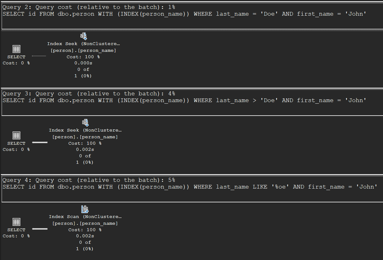
8. Index Examples and Tradeoffs (July 13, 2006)
This is the article where everything from June clicks together. The optimizer chooses an “access path” per table by weighing four questions: how many I/Os will a seek or scan cost, are the index keys usable for a predicate, how selective is that predicate, and does the index cover all the columns the query needs? Craig demonstrates each factor on a 100,000-row table, and the numbers do the teaching:
- I/O: for a query without a WHERE clause, scanning a narrow non-clustered index beats scanning the wide clustered index by almost a factor of nine in logical reads (the fat
char(200)column lives only in the clustered index) — easy to verify yourself withSET STATISTICS IO ONand an index hint. - Selectivity: with two candidate indexes for two range predicates, the optimizer seeks with the predicate that qualifies 9 rows and checks the other predicate as a residual, rather than the one that qualifies 99 rows.
- Seek vs. scan: the same query pattern flips from a clustered index seek to a non-clustered index scan when the range grows from ~8% to ~90% of the table — at that point scanning 174 pages beats touching 2,500.
- Lookup vs. scan: a seek plus bookmark lookup wins at 100 qualifying rows, but at 1,000 rows — still only 1% of the table! — the optimizer already prefers a full clustered index scan, because 1,000 random I/Os cost more than 2,800 sequential ones.
The I/O difference, measured on the 100,000-row table from the setup — the Messages tab shows 3,046 logical reads for the clustered index scan against 349 for the narrow index:
SET STATISTICS IO ON;
SELECT a, b FROM dbo.T WITH (INDEX(Ta));
SELECT a, b FROM dbo.T WITH (INDEX(Tb));
SET STATISTICS IO OFF;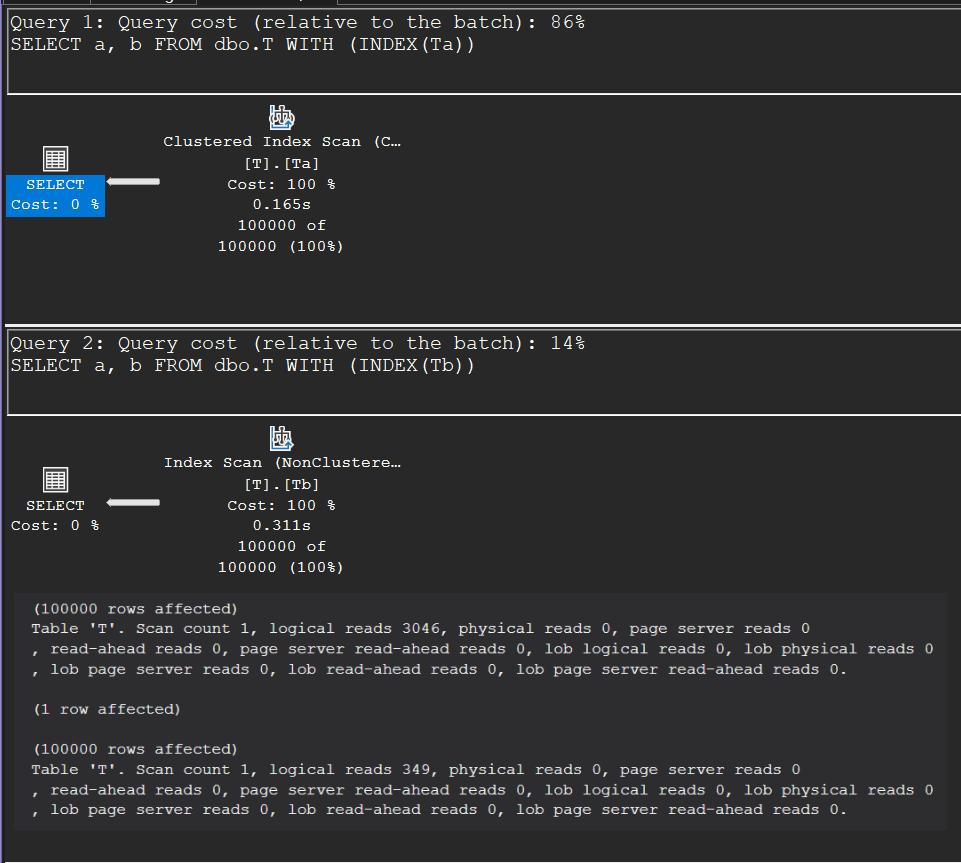
The seek-vs-scan flip, same table. At 8% of the rows the optimizer seeks the clustered index; at 90% it prefers scanning the narrow Tb index and gets the a column from the appended clustering key:
SELECT a FROM dbo.T WHERE a BETWEEN 1001 AND 9000;
SELECT a FROM dbo.T WHERE a BETWEEN 101 AND 90000;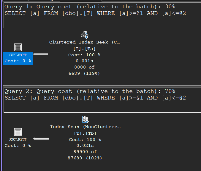
And the lookup-vs-scan flip. At 100 qualifying rows: Index Seek plus Key Lookup. At 1,000 rows — 1% of the table — the optimizer walks away from the index entirely (note the missing-index hint SSMS adds, suggesting a covering index that would win at both sizes):
SELECT x FROM dbo.T WHERE b BETWEEN 101 AND 200;
SELECT x FROM dbo.T WHERE b BETWEEN 1001 AND 2000;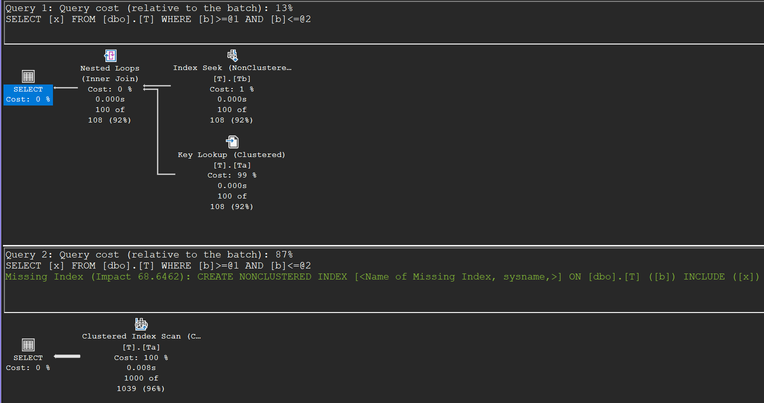
That last flip is the one to remember next time you wonder why SQL Server “ignores” your index.
9. Introduction to Joins (July 19, 2006)
The start of the join series, and a masterclass in keeping logical and physical concepts apart. Using a tiny Customers/Sales dataset, Craig walks through every logical join type SQL Server knows: inner join, the outer joins (left, right, full — with the unmatched rows “NULL extended”), cross join, the then-new CROSS APPLY/OUTER APPLY for joining against a table-valued function with a per-row parameter, and finally the two that have no T-SQL syntax of their own: the semi-join and anti-semi-join. Those last two are what actually show up in your plans when you write EXISTS or NOT EXISTS — a semi-join returns each qualifying row once, no matter how many matches it has, which is exactly the semantics you want from EXISTS.
You can see that on Craig’s own mini-dataset from the setup: the EXISTS becomes a Nested Loops (Left Semi Join), and the join produces 2 rows even though those customers have 3 matching sales between them:
SELECT *
FROM dbo.Customers AS C
WHERE EXISTS (SELECT * FROM dbo.Sales AS S WHERE S.Cust_Id = C.Cust_Id);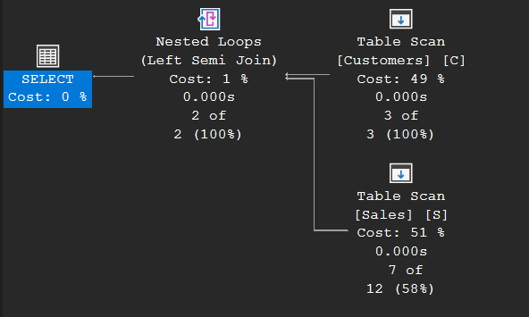
Two closing observations carry a lot of practical weight: equijoins (joins on equality) give the optimizer far more options than inequality joins, and inner joins give it more freedom to reorder than outer joins or applies do. In other words, the way you phrase a join constrains the plans the optimizer is even allowed to consider.
10. Nested Loops Join (July 26, 2006)
The first of the three physical join operators (nested loops, merge, hash). The algorithm is two nested for-loops: for each row from the outer input, scan the inner input for rows that satisfy the join predicate — which is why the naive cost is outer size × inner size. The interesting part is what an index does to that math: put an index on the inner table’s join key and each pass becomes a seek that returns only matching rows. The seek then depends on a value from the outer row (a “correlated parameter”, shown as OUTER REFERENCES in the plan), and you have what Craig calls an index join — the shape you see in OLTP plans everywhere.
Both shapes, side by side. First the naive algorithm — no indexes, so every outer row triggers a full Table Scan of the inner table (the OPTION (LOOP JOIN) hint keeps the optimizer from picking another join type on these tiny tables):
SELECT *
FROM dbo.Sales AS S
INNER JOIN dbo.Customers AS C ON S.Cust_Id = C.Cust_Id
OPTION (LOOP JOIN);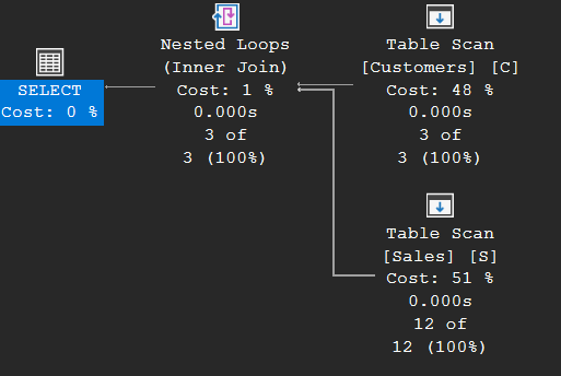
Now add an index on the inner join key and run the same query: the inner side becomes a Clustered Index Seek driven by the outer row’s Cust_Id — Craig’s “index join”. Click the Nested Loops operator and you’ll find the correlated parameter under OUTER REFERENCES:
CREATE CLUSTERED INDEX CI ON dbo.Sales (Cust_Id);
SELECT *
FROM dbo.Sales AS S
INNER JOIN dbo.Customers AS C ON S.Cust_Id = C.Cust_Id
OPTION (LOOP JOIN);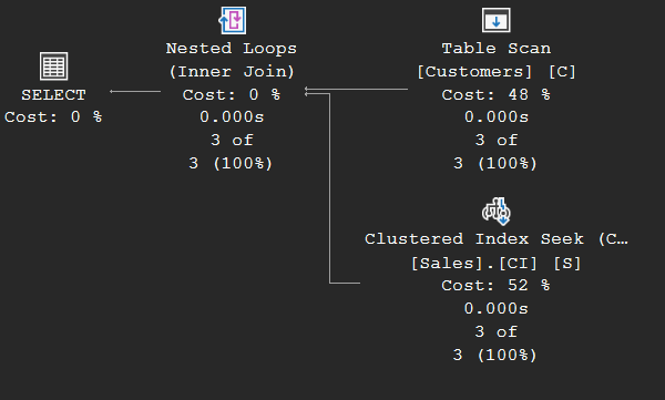
He also answers a question most people never think to ask: why do nested loops plans only come in “left” flavors? Left outer, left semi and left anti-semi join are trivial extensions of the loop; but a right outer join can’t work, because the inner table is read many times and some inner rows may never be visited at all when an index seek skips them. SQL Server solves this by commuting right joins into left joins, and builds a full outer join as a left outer join concatenated with an anti-semi-join for the leftovers. And the answer to “is nested loops good or bad?” is the one that applies to all three join operators: neither — it shines with small outer inputs and an indexed inner key, and it is sometimes the only option, such as for cross joins or joins without any equality predicate. Merge join and hash join are up next, in the August articles.
Done experimenting? This removes everything the setup created:
-- Cleanup
DROP TABLE IF EXISTS dbo.person, dbo.T, dbo.Customers, dbo.Sales;