

Part 3 of my series on Craig Freedman’s classic SQL Server query-processing blog (part 2, July 2006, is here). August 2006 was join month: the two remaining physical join operators, a summary that pits all three against each other, and then two articles showing how the optimizer uses joins for something you might not expect — subqueries. As always, I summarize each article in my own words; everything still applies to modern SQL Server versions.
All plan screenshots in this post are my own, made in SSMS with “Include Actual Execution Plan” (Ctrl+M). Want to follow along? Run this one-time setup in a scratch database (it uses GENERATE_SERIES, so SQL Server 2022 or later) — the cleanup is at the bottom of the post:
-- One-time setup for the examples in this post
CREATE TABLE dbo.T1 (a INT, b INT, x CHAR(200));
CREATE TABLE dbo.T2 (a INT, b INT, x CHAR(200));
INSERT dbo.T1 SELECT value * 2, value * 5, value FROM GENERATE_SERIES(0, 999);
INSERT dbo.T2 SELECT value * 3, value * 7, value FROM GENERATE_SERIES(0, 999);

CREATE TABLE dbo.T1h (a INT, b INT, x CHAR(200));
CREATE TABLE dbo.T2h (a INT, b INT, x CHAR(200));
INSERT dbo.T1h SELECT value * 2, value * 5, value FROM GENERATE_SERIES(0, 999);
INSERT dbo.T2h SELECT value * 3, value * 7, value FROM GENERATE_SERIES(0, 9999);

CREATE TABLE dbo.T3 (a INT, b INT, x CHAR(200));
INSERT dbo.T3 SELECT value * 5, value * 11, value FROM GENERATE_SERIES(0, 99999);

CREATE TABLE dbo.T4 (a INT, b INT, c INT);
CREATE TABLE dbo.T5 (a INT UNIQUE CLUSTERED, b INT);
INSERT dbo.T4 VALUES (0, 0, 0), (1, 1, 1);11. Merge Join (August 3, 2006)
The second physical join operator has two entry requirements: at least one equality (equijoin) predicate, and both inputs sorted on the join keys. In return you get a beautiful property: each input is read once, so the cost is proportional to the sum of the input sizes instead of the product — which is why merge join scales to larger inputs than nested loops. The sort order can come from an explicit Sort operator or, much cheaper, from an index.
Without any indexes the optimizer wouldn’t choose merge here on its own — the hint forces it, and both requirements become visible in the plan: an explicit Sort on each input, and (in the operator’s tooltip) the many-to-many flag, since nothing proves either side unique:
SELECT * FROM dbo.T1 JOIN dbo.T2 ON T1.a = T2.a OPTION (MERGE JOIN);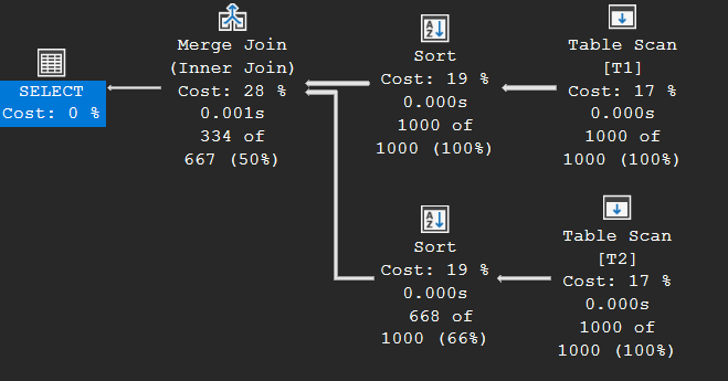
The distinction worth remembering from this article is one-to-many versus many-to-many. If the optimizer can prove one input is unique (a unique index, or a distinct/group-by in the plan), it can discard rows as it goes. If not, it must buffer duplicate join keys in a worktable in tempdb so it can replay them — visible as the MANY-TO-MANY keyword in the plan, and always more expensive. Craig’s examples show nice subtleties: a merge join can quit early once one sorted input is exhausted, and a unique single-column index can even provide order on two columns, because within one unique key value any appended column is trivially “sorted”.
Create unique clustered indexes on the join keys and run the same join again, this time without a hint: the optimizer now picks merge join voluntarily. Both Sorts are gone (the indexes deliver the order), and the unique index on T2(a) turns it into a one-to-many join — no tempdb worktable needed:
CREATE UNIQUE CLUSTERED INDEX T1ab ON dbo.T1 (a, b);
CREATE UNIQUE CLUSTERED INDEX T2a  ON dbo.T2 (a);

SELECT * FROM dbo.T1 JOIN dbo.T2 ON T1.a = T2.a;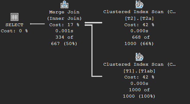
12. Hash Join (August 10, 2006)
The heavy lifter. Hash join works in two phases: build (read the first input completely and build an in-memory hash table on the join keys — the optimizer tries to put the smaller input here) and probe (stream the second input past that hash table). Like merge join it demands an equijoin predicate; unlike merge join it needs no sort order, which makes it the default choice for large, unindexed inputs and data-warehouse work.
Join a 1,000-row heap to a 10,000-row heap and hash join is exactly what you get, no hint required — with the small table on top as the build input:
SELECT * FROM dbo.T1h JOIN dbo.T2h ON T1h.a = T2h.a;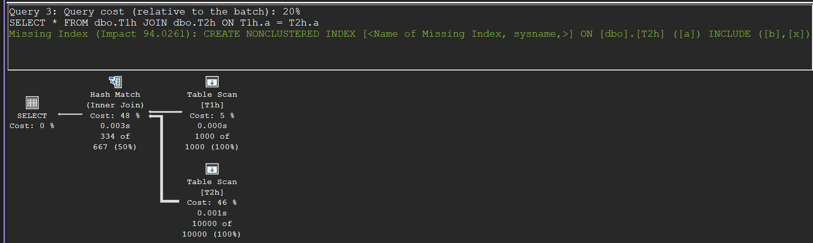
The costs are the flip side: hash join is blocking on its build input and needs a memory grant sized from the cardinality estimate. Underestimate it, and the join spills partitions of the hash table to tempdb — the spill mechanism is described here in detail, years before “hash spill” warnings appeared in the plan XML. The article’s most underrated section explains left-deep versus right-deep hash join trees: in a left-deep tree only adjacent joins are active at once and can share memory, while in a right-deep tree all hash tables must exist simultaneously — and Craig shows the optimizer switching shapes purely based on input sizes.
Here is the right-deep case reproduced: a filter makes both small tables tiny, so the optimizer builds a hash table on each of them and lets the 100,000-row T3 stream through both joins as the probe input:
SELECT * FROM (dbo.T1h JOIN dbo.T2h ON T1h.a = T2h.a) JOIN dbo.T3 ON T1h.b = T3.a
WHERE T1h.a < 100;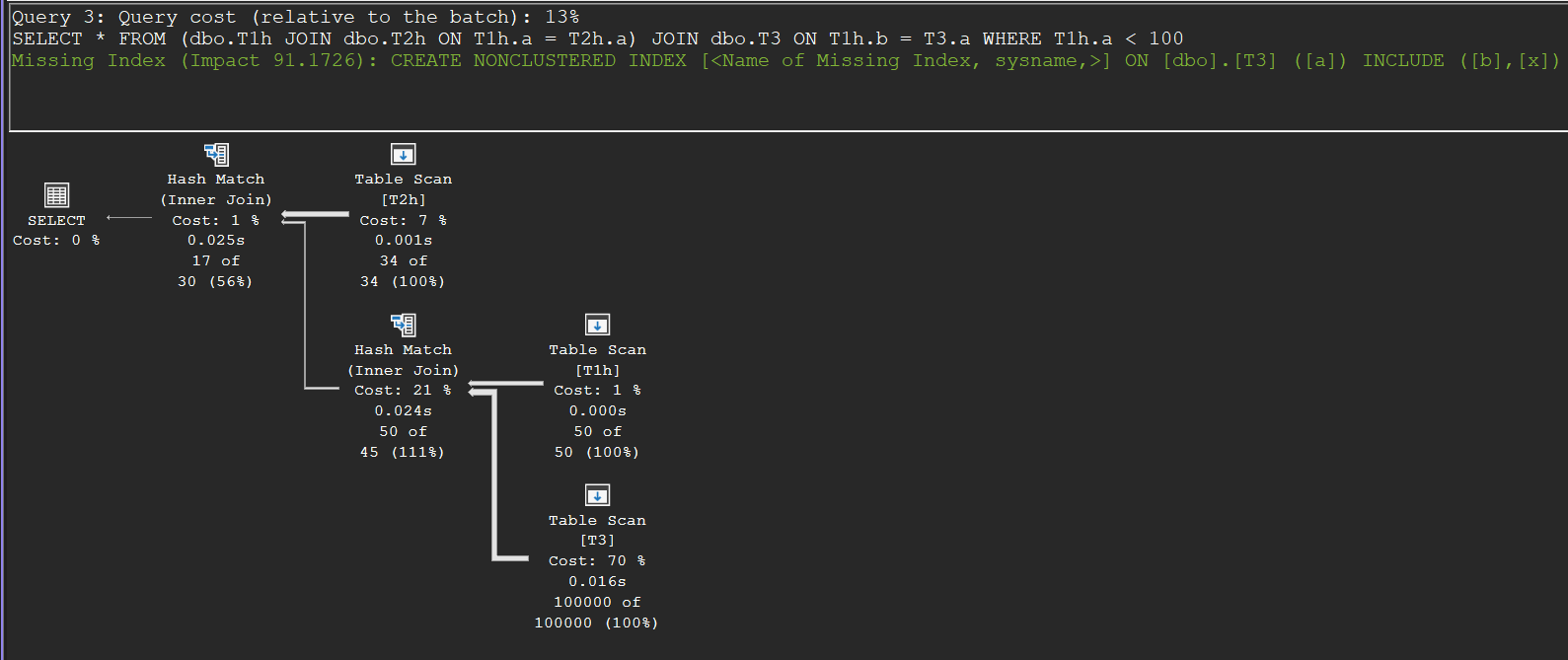
13. Summary of Join Properties (August 16, 2006)
The reference card for the whole join series. In short:
| Nested Loops | Merge | Hash | |
|---|---|---|---|
| Sweet spot | small outer input + index on inner join key | medium/large sorted inputs, or when order is needed anyway | large unsorted inputs, DW/parallel workloads |
| Equijoin required | no | yes* | yes |
| Blocking | no | no | build input only |
| Memory grant | no | no (its sorts might) | yes |
| Preserves order | outer input only | yes | no |
The second half demonstrates how fragile the choice is: the same two 1,000-row tables produce a hash join plain, a nested loops join with TOP 10, a merge join with TOP 100 or an ORDER BY, back to hash when a filter shrinks one input, and loops again when the filter lands on the other side. It closes with the join hints (LOOP/MERGE/HASH JOIN, FORCE ORDER) — recommended only for experimentation, with a warning about error 8622 when the hinted plan can’t exist.
An honest footnote from trying to reproduce this twenty years later: on my SQL Server 2022 instance the join type refuses to flip — plain, TOP 10 and TOP 100 all stay Hash Match. But look at the Table Scan of T2h in the actual plans below: 10,000 rows read without TOP, only 19 with TOP 10 and 199 with TOP 100. The row goal machinery Craig describes is alive and well; today’s cost model just answers it inside the same join type. A nice reminder that his plans are teaching examples, not guarantees:
SELECT *         FROM dbo.T1h JOIN dbo.T2h ON T1h.a = T2h.a;
SELECT TOP 10 *  FROM dbo.T1h JOIN dbo.T2h ON T1h.a = T2h.a;
SELECT TOP 100 * FROM dbo.T1h JOIN dbo.T2h ON T1h.a = T2h.a;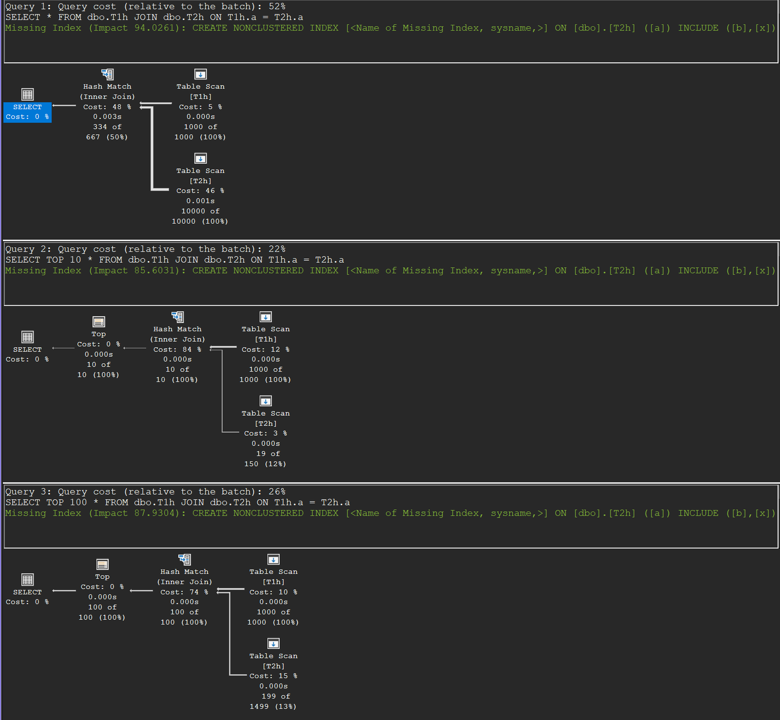
14. Subqueries in CASE Expressions (August 23, 2006)
What happens when a CASE expression contains subqueries? Two pieces of exotic join machinery appear. An EXISTS in the WHEN clause becomes a semi-join with a probe column: unlike a normal semi-join it returns every outer row and just records true/false in the probe column, so the CASE can pick a branch per row. A subquery in the THEN or ELSE clause becomes a nested loops join with a passthru predicate: if the predicate is true the row passes straight through and the inner side is never executed — SQL Server’s way of guaranteeing the subquery only runs for rows where that branch is actually taken.
That leads to a diagnostic gem: a passthru predicate is the only case where the row count on the outer side of a nested loops join doesn’t match the number of executes on the inner side. Multiple WHEN branches simply chain these joins with increasingly clever passthru conditions.
Both pieces of machinery in one plan, on two tiny tables. The semi-join with the probe column sits on the right, the outer join with the passthru predicate to its left; click either seek on T5 and compare its number of executions with the two outer rows to see the branches being skipped:
SELECT CASE
         WHEN EXISTS (SELECT * FROM dbo.T5 WHERE T5.a = T4.a)
           THEN (SELECT T5.b FROM dbo.T5 WHERE T5.a = T4.b)
         ELSE T4.c
       END
FROM dbo.T4;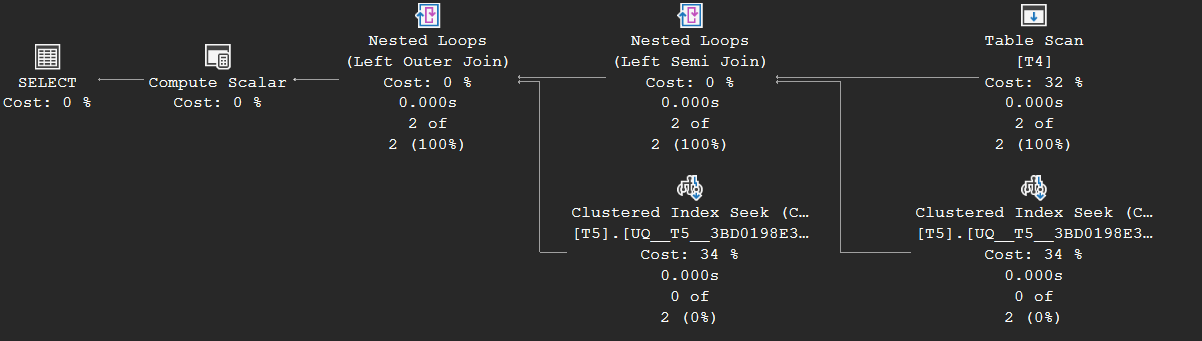
15. Subqueries: ANDs and ORs (August 30, 2006)
Combining EXISTS/NOT EXISTS subqueries with AND is easy: the plan just stacks semi-joins and anti-semi-joins in sequence. OR is the interesting case, because a row must survive if either subquery matches. The optimizer has two strategies: feed the union of both subqueries into a single semi-join (a Concatenation under the join), or run two separate semi-joins and deduplicate the combined result — using an internal unique row key, so it works even when the table has no unique key of its own. A NOT EXISTS inside an OR gets inverted through a Constant Scan trick that turns “no match found” into “row produced”.
The first strategy in action: one Nested Loops (Left Semi Join) whose inner input is a Concatenation of the two subquery seeks — either match lets the outer row survive:
SELECT * FROM dbo.T4
WHERE EXISTS (SELECT * FROM dbo.T5 WHERE T5.a = T4.a)
   OR EXISTS (SELECT * FROM dbo.T5 WHERE T5.a = T4.b);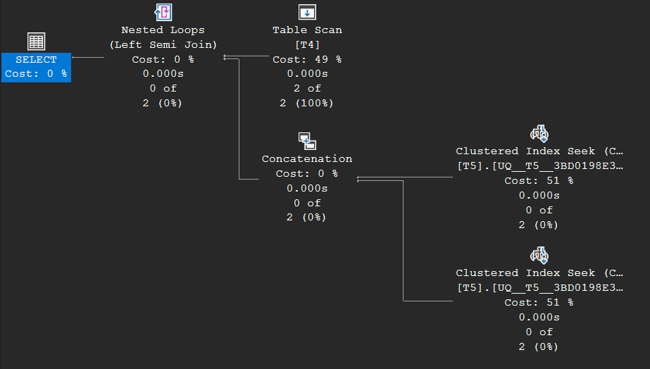
The closing performance note deserves a highlight: nested loops semi-joins can be erratic, because they stop at the first match — fast when a match is found early, painfully slow when there is none and the whole inner input must be searched. Same plan, wildly different performance, small change in data. The cure, as usual: the right indexes.
Done experimenting? This removes everything the setup created:
-- Cleanup
DROP TABLE IF EXISTS dbo.T1, dbo.T2, dbo.T3, dbo.T1h, dbo.T2h, dbo.T4, dbo.T5;